ARMA and ARIMA Timeseries Prediction With Python and Pandas

In this article I will try to give a brief introduction on how to make timeseries prediction with Python. For brevity I will try to skip the theory of timeseries. If you need to understand about timeseries please google the different terms that I used in this tutorial. So, without any delay lets start to code.

I this article I used Pandas which is a very popular python library for statistics. First let add following lines at the top of our python file. It will import all the required library for our purpose.

import numpy as np
import pandas as pd
import matplotlib.pyplot as plt
from statsmodels.tsa.arima_model import ARMA, ARIMA
from statsmodels.tsa.stattools import adfuller, arma_order_select_ic

In this tutorials we used the dataset from kaggle which has the average temperature of the different countries of the world. It includes both land and sea temperature. Database is quite large so we will only pick one country to predict temperature. We will pick Canada.

Your can download the dataset from this link: Climate Change: Earth Surface Temperature Data

File is in csv format so first we have to read data from csv file using following code.

df = pd.read_csv('GlobalLandTemperaturesByCountry.csv',                 
                   sep=',',                 
                   skipinitialspace=True,                 
                   encoding='utf-8')

Our initial data will contain many unwanted values. We must clean them with care otherwise they will create unexpected results. To to this:

df = df.drop('AverageTemperatureUncertainty', axis=1)
df = df[df.Country == 'Canada']
df = df.drop('Country', axis=1)
df = df[df.AverageTemperature.notnull()]

df.index = pd.to_datetime(df.dt)
df = df.drop('dt', axis=1)
df = df.ix['1900-01-01':]
df = df.sort_index()
df.AverageTemperature.fillna(method='pad', inplace=True)

See, we dropped all null values from our pandas dataframe object. Also notice, we have only picked our values from the beginning of 1900. Because large data take very long time to calculate and sometimes gives error message from code which could be very annoying for a novice like me.

At this point you might want to see how the plot looks like. Here is the code for that:

plt.plot(df.AverageTemperature)
plt.show()

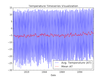
Now lets see the moving average of our timeseries data.

# Rolling Mean/Moving Average
df.AverageTemperature.plot.line(style='b', legend=True, grid=True, 
                                 label='Avg. Temperature (AT)')
ax = df.AverageTemperature.rolling(window=12).mean().plot.line(style='r', 
                                   legend=True, label='Mean AT')
ax.set_xlabel('Date')
plt.legend(loc='best')
plt.title('Temperature Timeseries Visualization')
plt.show()

To make a prediction from a timeseries the data has to stationary. To check the stationarity of data we will use Dickey–Fuller test. Here is the code for this -

def stationarity_test(df):
    print 'Results of Dickey-Fuller Test:'    dftest = adfuller(df)
    indices = ['Test Statistic', 'p-value',
            'No. Lags Used', 'Number of Observations Used']
    output = pd.Series(dftest[0:4], index=indices)
    for key, value in dftest[4].items():
        output['Critical Value (%s)' % key] = value
    print output

stationarity_test(df.AverageTemperature)

====================================================================
                        STATIONARITY TEST
====================================================================
Results of Dickey-Fuller Test:
Test Statistic                   -3.991544
p-value                           0.001455
No. Lags Used                    24.000000
Number of Observations Used    1340.000000
Critical Value (5%)              -2.863699
Critical Value (1%)              -3.435239
Critical Value (10%)             -2.567920
dtype: float64

Test shows our data is stationary. Now we are ready for doing our prediction. I will show both ARMA and ARIMA prediction one after another.

Autoregressive–moving-average model

From Wikipedia, In the statistical analysis of time series, autoregressive–moving-average (ARMA) models provide a parsimonious description of a (weakly) stationary stochastic process in terms of two polynomials, one for the autoregression and the second for the moving average. The general ARMA model was described in the 1951 thesis of Peter Whittle, Hypothesis testing in time series analysis, and it was popularized in the 1971 book by George E. P. Box and Gwilym Jenkins.

Given a time series of data Xt , the ARMA model is a tool for understanding and, perhaps, predicting future values in this series. The model consists of two parts, an autoregressive (AR) part and a moving average (MA) part. The AR part involves regressing the variable on its own lagged (i.e., past) values. The MA part involves modeling the error term as a linear combination of error terms occurring contemporaneously and at various times in the past.

The model is usually referred to as the ARMA(p,q) model where p is the order of the autoregressive part and q is the order of the moving average part.

Determining this p and q value can be a challenge. So, pandas has a function for finding this. To get the p and q value -

print arma_order_select_ic(df.AverageTemperature, 
         ic=['aic', 'bic'], trend='nc', 
         max_ar=4, max_ma=4, 
         fit_kw={'method': 'css-mle'})

{'bic_min_order': (3, 3), 'aic_min_order': (3, 3), 'bic':              0            1            2            3            4
0          NaN  9551.833892  8627.365113  8074.089428  7696.441328
1  9055.274290  8272.865241  7839.717253  8535.844196  8010.958470
2  7069.951373          NaN  6633.176005  6500.003441  6380.696664
3  6836.470928  6838.489737          NaN  5255.494118          NaN
4  6829.801936  6849.877710          NaN          NaN          NaN, 'aic':              0            1            2            3            4
0          NaN  9541.396072  8611.708384  8053.213790  7670.346779
1  9044.836471  8257.208512  7818.841614  8509.749647  7979.645012
2  7054.294644          NaN  6607.081457  6468.689982  6344.164296
3  6815.595289  6812.395189          NaN  5218.961750          NaN
4  6803.707387  6818.564252          NaN          NaN          NaN}

The commented line showing the result we have found. p=3, q=3. Great!!!

Lets fit the model and make prediction using ARMA.

# Fit the modelts = pd.Series(df.AverageTemperature, index=df.index)
model = ARMA(ts, order=(3, 3))
results = model.fit(trend='nc', method='css-mle', disp=-1)
print(results.summary2())

Results: ARMA
========================================================================
Model:                ARMA                 BIC:                   5255.4941
Dependent Variable:   AverageTemperature   Log-Likelihood:        -2602.5
Date:                 2016-08-25 03:09     Scale:                 1.0000  
No. Observations:     1365                 Method:                css-mle
Df Model:             6                    Sample:                01-01-1900
Df Residuals:         1359                                        09-01-2013
Converged:            0.0000               S.D. of innovations:   1.621  
AIC:                  5218.9618            HQIC:                  5232.636
----------------------------------------------------------------------------
                          Coef.  Std.Err.      t      P>|t|   [0.025  0.975]
----------------------------------------------------------------------------
ar.L1.AverageTemperature  2.7314   0.0001  30937.6060 0.0000  2.7312  2.7316
ar.L2.AverageTemperature -2.7309   0.0001 -20632.3816 0.0000 -2.7311 -2.7306
ar.L3.AverageTemperature  0.9993   0.0001  14429.0528 0.0000  0.9992  0.9995
ma.L1.AverageTemperature -2.6400   0.0227   -116.1775 0.0000 -2.6845 -2.5954
ma.L2.AverageTemperature  2.5567   0.0393     65.0647 0.0000  2.4797  2.6337
ma.L3.AverageTemperature -0.8950   0.0221    -40.4167 0.0000 -0.9384 -0.8516
----------------------------------------------------------------------------------------
                   Real              Imaginary             Modulus             Frequency
----------------------------------------------------------------------------------------
AR.1              1.0006               -0.0000              1.0006               -0.0000
AR.2              0.8661               -0.5000              1.0001               -0.0833
AR.3              0.8661                0.5000              1.0001                0.0833
MA.1              0.8815               -0.4946              1.0108               -0.0814
MA.2              0.8815                0.4946              1.0108                0.0814
MA.3              1.0936               -0.0000              1.0936               -0.0000
=======================================================================
Now, plot the prediction -

# Plot the modelfig, ax = plt.subplots(figsize=(10, 8))
fig = results.plot_predict('01/01/2010', '12/01/2023', ax=ax)
ax.legend(loc='lower left')
plt.title('Temperature Timeseries Prediction')
plt.show()

predictions = results.predict('01/01/2010', '12/01/2016')

OK. At this point we have successfully predicted from our time series data.
Autoregressive integrated moving average

Again from Wikipedia, in statistics and econometrics, and in particular in time series analysis, an autoregressive integrated moving average (ARIMA) model is a generalization of an autoregressive moving average (ARMA) model. Both of these models are fitted to time series data either to better understand the data or to predict future points in the series (forecasting). ARIMA models are applied in some cases where data show evidence of non-stationarity, where an initial differencing step (corresponding to the "integrated" part of the model) can be applied to reduce the non-stationarity.[1]

The AR part of ARIMA indicates that the evolving variable of interest is regressed on its own lagged (i.e., prior) values. The MA part indicates that the regression error is actually a linear combination of error terms whose values occurred contemporaneously and at various times in the past. The I (for "integrated") indicates that the data values have been replaced with the difference between their values and the previous values (and this differencing process may have been performed more than once). The purpose of each of these features is to make the model fit the data as well as possible.

Non-seasonal ARIMA models are generally denoted ARIMA(p,d,q) where parameters p, d, and q are non-negative integers, p is the order (number of time lags) of the autoregressive model, d is the degree of differencing (the number of times the data have had past values subtracted), and q is the order of the moving-average model. Seasonal ARIMA models are usually denoted ARIMA(p,d,q)(P,D,Q)m, where m refers to the number of periods in each season, and the uppercase P,D,Q refer to the autoregressive, differencing, and moving average terms for the seasonal part of the ARIMA model.[2][3]

When two out of the three terms are zeros, the model may be referred to based on the non-zero parameter, dropping "AR", "I" or "MA" from the acronym describing the model. For example, ARIMA (1,0,0) is AR(1), ARIMA(0,1,0) is I(1), and ARIMA(0,0,1) is MA(1).

Lets predict using another method called ARIMA which is also very popular approach. If you look closely then you will see I used q value 4. I did this because pandas will show error if you use p and q as same value. So, I chose 4. So, lets get going - 

# Fit the model ARIMAmodel_arima = ARIMA(ts, order=(3, 1, 4))
results_arima = model_arima.fit(disp=-1, transparams=True)
print(results_arima.summary2())

# Plot the modelfig, ax = plt.subplots(figsize=(10, 8))
fig = results_arima.plot_predict('01/01/2010', '12/01/2016', ax=ax)
ax.legend(loc='lower left')
plt.title('Temperature Timeseries Prediction')
plt.show()

predictions = results_arima.predict('01/01/2010', '12/01/2016')

                               Results: ARIMA
=============================================================================
Model:                 ARIMA                 Log-Likelihood:       -2617.8
Dependent Variable:    D.AverageTemperature  Scale:                1.0000  
Date:                  2016-08-25 03:09      Method:               css-mle
No. Observations:      1364                  Sample:               02-01-1900
Df Model:              8                                           09-01-2013
Df Residuals:          1356                  S.D. of innovations:  1.637  
AIC:                   5253.6783             HQIC:                 5271.257
BIC:                   5300.6418                                          
-----------------------------------------------------------------------------
                            Coef.  Std.Err.     t      P>|t|   [0.025  0.975]
-----------------------------------------------------------------------------
const                      -0.0009   0.0000  -857.2900 0.0000 -0.0009 -0.0009
ar.L1.D.AverageTemperature  0.7466   0.0001 11452.3450 0.0000  0.7465  0.7467
ar.L2.D.AverageTemperature  0.7065   0.0001 11071.5117 0.0000  0.7063  0.7066
ar.L3.D.AverageTemperature -0.9853      nan        nan    nan     nan     nan
ma.L1.D.AverageTemperature -1.4480   0.0581   -24.9265 0.0000 -1.5619 -1.3342
ma.L2.D.AverageTemperature -0.2202   0.0552    -3.9898 0.0001 -0.3284 -0.1120
ma.L3.D.AverageTemperature  1.4560   0.0676    21.5279 0.0000  1.3235  1.5886
ma.L4.D.AverageTemperature -0.7053   0.0468   -15.0849 0.0000 -0.7970 -0.6137
-----------------------------------------------------------------------------------------
                    Real              Imaginary             Modulus             Frequency
-----------------------------------------------------------------------------------------
AR.1              -1.0149               -0.0000              1.0149               -0.5000
AR.2               0.8660               -0.5001              1.0000               -0.0834
AR.3               0.8660                0.5001              1.0000                0.0834
MA.1              -1.0106               -0.0000              1.0106               -0.5000
MA.2               0.9386               -0.5389              1.0823               -0.0829
MA.3               0.9386                0.5389              1.0823                0.0829
MA.4               1.1976               -0.0000              1.1976               -0.0000
=============================================================================


So, that's the end. We have successfully predicted timeseries using both ARMA and ARIMA.